Project Timeline

Our semester long project proceeded in the following chronological order

1. August/September - collect data and formulate a well defined problem statement
2. October - Explore various segmentation methods to identify feature edges in micrographs
3. November - Develop relevant statistics based on calculating chord length distributions. Begin data reduction in PC space. Some other exploratory statistics that failed (see below).
4. December - Finalize data reduction tasks in PC space. Explore machine learning possibilities from given data set. Develop visualizations and presentation.

Work Load Distribution

• Data collection (Patxi)
• Image processing, cropping, alignment (Ahmet)
• Edge detection (Patxi/Ahmet)
• Chord length distribution (Patxi/Ahmet)
• PC reduction (Patxi/Ahmet)
• Machine Learning (Ahmet)
• Data visualization (Patxi/Ahmet)

Machining Introduction

Machining is a secondary manufacturing operation that typically follows primary shaping processes such as casting or forging. Imposed strains and strain rates can be as large as 10^5 1/s and 1-15, respectively. During these extreme deformation conditions significant energy is dissipated through plastic work which increases the temperatures in the chip.

The described strain-rate-temperature conditions define a thermomechanical processing route that is unique to machining.

Measured shear strain rates for oxygen-free high-conductivity (OFHC) copper. Note that velocimetry techniques are limited to lower machining speeds; in this case a 0.01 m/s speed was utilized. Industrial applications maching at 3-5 m/s where strain rates may approach 10^5 1/s.

Measured shear strains for this set of experiments fall in the 3-12 range.

Processing Effects on Microstructure

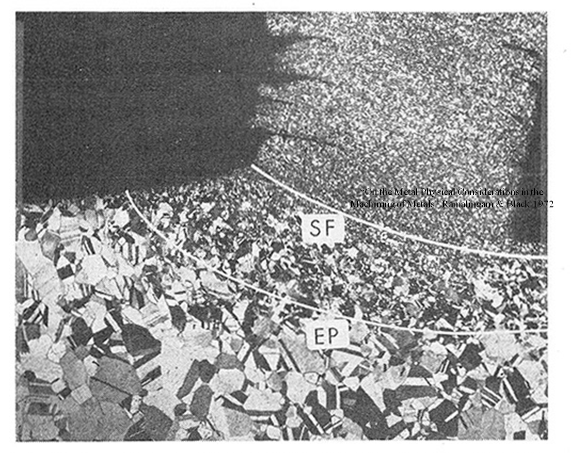
The imposed thermomechanical processing route can induce significant microstructural changes in both the machined workpiece and the produced chip. Microstructural changes may include but are not limited to,

• Grain refinement
• Increase in dislocation density
• Increase in twin density

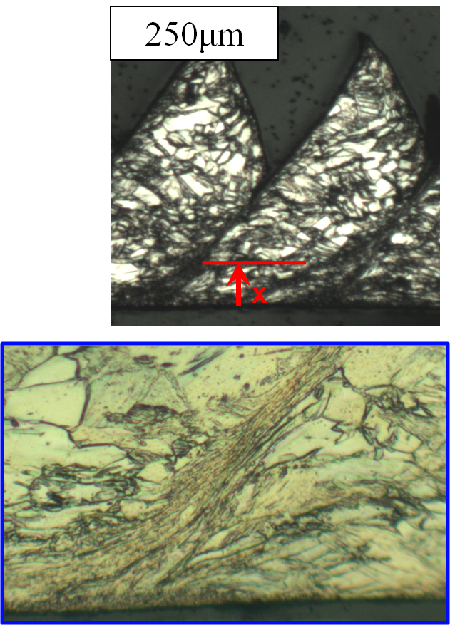
Micrograph from a quick-stop machining experiment displaying the gradation of structure in brass from the relatively undeformed bulk to the highly refined chip.

TEM work showing features on the nanometer length scale.

Problem Statement

The manufacturing community has begun to investigate linkages between processing and structure in machining. The motivation is that designers can produce better components if surface structure is tailored for specific applications; highly refined grain structure could be beneficial for fretting applications but deleterious in a corrosive environment.

The goal of the present work is to explore process-structure linkages in priciple component (PC) space while quantifying structure gradients present in machined chips. Gradients in the direction perpendicular to the machined surface will be addressed. 7 unique processing conditions will be utilized. The structure we are addressing are grain boundaries.

Experimental

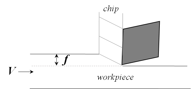
The orthogonal cutting model is 2D a experimental technique that assumes a plane strain condition in the depth direction. Experiments can be performed that approximate this condition and are valuable as they simplify geometry such that 2D inspection of the microstructure is sufficient to characterize the chip or workpiece.

The two independent experimental variables in this configuration are

• feed (f)
• cutting velocity (V)

These variables control the imposed strains, rates and temperature and as such they have a direct effect on the final structure of the chips.

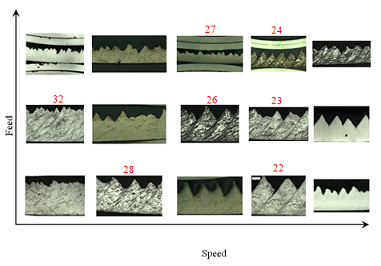
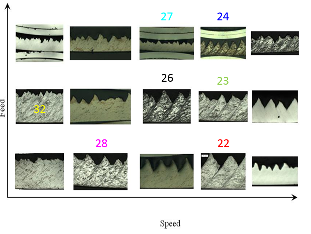
A number of experiments were performed across three feeds and five speeds. Samples were prepared metallographically and etched. A total of 7 samples were used for this study. 5 images of separate chip ‘segments’ were used as the data set for each processing condition. The assumption is that each individual ‘segment’ is statistically representative of the imposed processing conditions.

Microstructure Segmentation

The following procedure was used to process, segment and develop chord-length distributions.

• Detect chip-epoxy interface in each sample
• rotate all images so that the chip-epoxy interface is aligned horizontally
• crop out a smaller image from the rotated images
• Convert to grayscale
• Filtering to remove noise
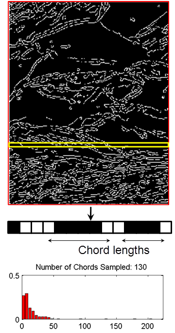
• Canny edge detection to identify edges (i.e. grain/phase boundaries)
• calculate length of chords in each row of image
• bin data using 1 pixel increments and develop PDF of chord length distribution from counts

Two different chord-length statistics were considered for this work

1. The probability that a chord in a row is of length X
2. The probability that a pixel in a row is found in a chord of length X

Each distribution in a sample image can be seen below.

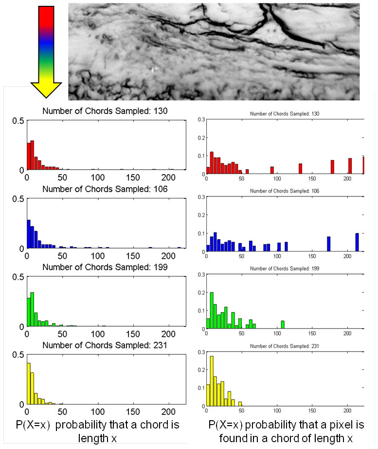
Note that the later definition does a much better job of describing the longer chord lengths away from the machined surface. This agrees with what is expected as larger grains are observed further away from the machined surface.

Attempt at Spatial statistics

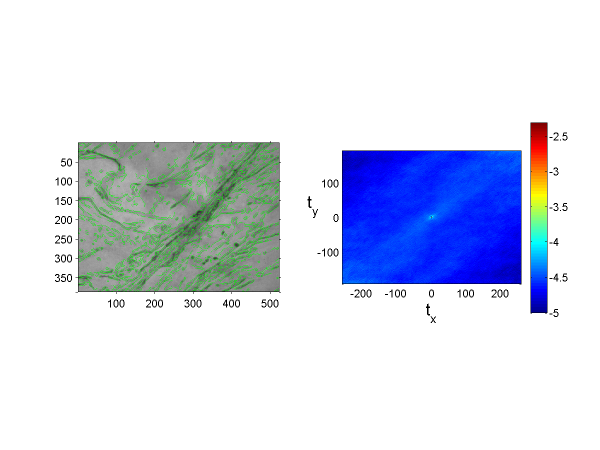
An attempt was made directly use the segmented binary images to generate spatial statistics. This was discussed in part in a blog posted on 11-04-2014.

The logarithm of the autocorrelation is shown below (nonperiodic boundary conditions). Note that as the images are large (more than 200,000 pixels) the volume fraction of edges is very low (1000s of edge pixels per image). As such a logarithmic transformation was used scale data prior to visualization (without this everything is blue…).

As expected the spatial distribution of the statistics does capture the orientation of the shear bands. The likelihood that both the tail and head of a vector fall on a edge pixel is highest along the direction of a shear band.

There are however a few concerns associated with quantitatively using these results,

1. How can we capture spatial gradients using this methodology? Should we discritize each image to a smaller image (100 x 100 pixels)? If we do this however we also constrain the length scales that can be represented in the spatial statistics (get a 100 x 100 autocorrelation map). It was not clear how to proceed forward given these maps.
2. The numbers associated with the autocorrelation map are on the order of 10^-3 to 10^-5. This is because we are identifying state 1 as a grain-interior and state 2 as a grain-boundary. As this is a pure titanium (only alpha phase is present) and we only have access to optical microscopy there is no better way to define states. It is difficult to be confident with the data and extract meaningful insight from these statistics.

As such it was decided that the chord length distributions should be used to quantify the microstructure rather than spatial statistics.

Data Reduction

Chord length distributions were developed across all rows of pixels in each image. Frequency of chord lengths were summed over all 5 images for each process condition. This represents the “averaged” data set.

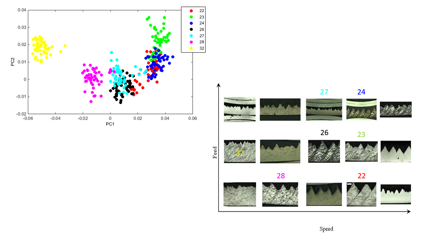
Principal Component Analsysis (PCA) was used to reduce the dimensionality of the problem. A plot of PC1 and PC2 in PC-space for the top 50 pixels are shown in the following image.

Note that there is some clustering associated with processing conditions. In particular clustering appears to most associated with cutting velocity.

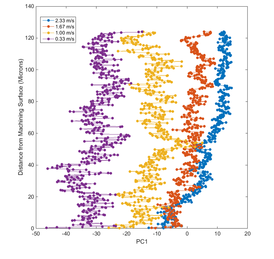
There appeared to be NO clustering of data in the bottom 50 pixels of each image (adjacent to the machined surface). It is very likely that the level of resolution needed to quantify structure in the zone exceeds the limitations of optical microscopy. PC1 is shown as a function of distance away from the machining surface below. Note that there is very clear clustering away from the machined surface but much more overlap at the surface.

Results

Machine Learning

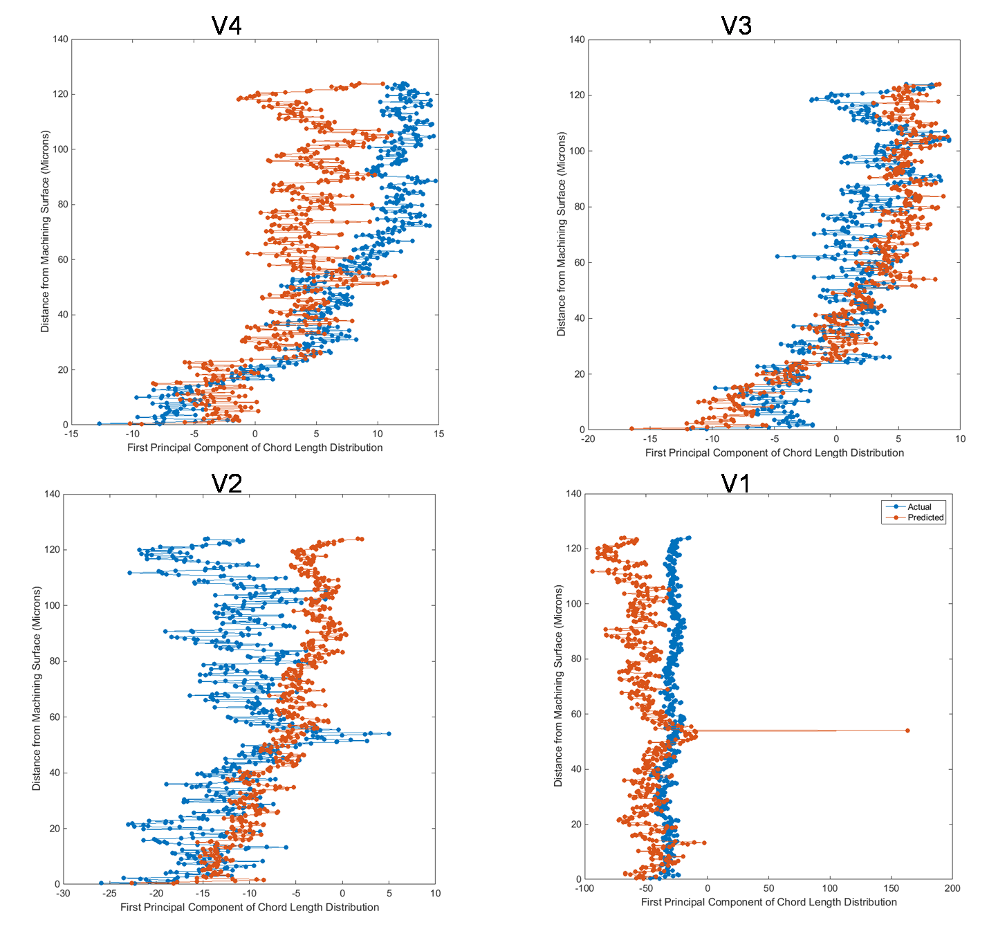
As an exercise we wanted to test the predictive capabilities of a trained model. As clustering appeared to be best captured by PC1 and the machining velocity (feed played less of a role) the produced data was averaged and marginalized over feeds for the four speeds tested.

Then we wanted to see if we can predict the average vertical gradient at a given speed, provided we know the gradients at the other three speed settings. A simple regression based predictive model was used to train on the known speed settings for every binned distance (or rows of pıxels) from the machining surface individually, meaning a markov property was assumed over the vertical gradient. Despite the crudeness of the model, the goal here was to showcase reasonably accurate estimates and the ability to obtain much better models if the data warrants it. As shown below, the estimates were reasonably accurate and can easily be improved with a more adaptive model. We did not explore any more sophisticated methods due to discovered inconsistencies ın the dataset.

Etch Gradients

A somewhat unexpected result was discovered associated with etching gradients present in machined chips.

While exploring PC1 data from processing condition #32 it was observed that data associated with each individual image was arranged in the same order that the images were taken.

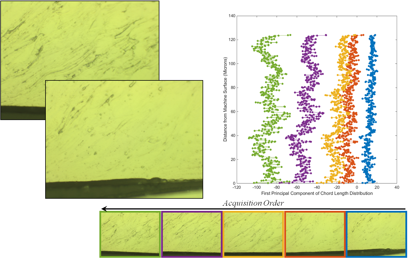
The images were taken by incrementally translating over the chip along the length of the chip. Incidentally, all chips have some degree of an etch gradient eminating from the center of the chip. The chip associated with processing condition #32 has the largest such gradient; towards the middle it appears as if the chip is completely unetched yet towards the ends it is etched.

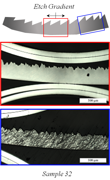
It is certainly possible that the identical polishing and etching technique could produce varying results in different chips as chips potentially contain varying degrees of work hardening and residual stresses. However it is unclear why etch gradients exist in individual chips. It is possible that polishing mechanics differ between the interior and edges due to the presence of stainless steel clips in the center (if say the holders are more resistive to the abrasion process and are slightly elevated relative to chip). Analogously a similar argument could explain why using a swabbing etching technique could preferentially etch material due to the presence of the clip holders (i.e. more pressure can be applied away from the clip while swabbing thus breaking up protective oxide layers).

Conclusions

• Current techniques are fairly successful in classifying the structure towards the inner parts of the chips for the current dataset.
• The current techniques cannot resolve information close to the machining surface as distinctly as the information farther away.
  • Grain refinement in the highly sheared zones may be on the nanometer length scale. Optical microscopy is limited to a few microns. It is very likely that insufficient quantification of the structure lead to poor classification near the machined surface interface.
• Uneven etching effects were found to be effectively captured by the principal components of chord length distribution.
• Process path learning was demonstrated with variable accuracy on the given dataset. Substantial improvements were possible, but not explored, due to the current limitations and amount of data.

Future Work

• More Reliable Imaging
• Different Polishing and Etching Techniques
  • Accounting for the Etching Gradients
  • Electropolishing
  • Eliminating SS clips or holding towards edge of chip
  • Different etchant
• SEM
  • Higher magnification
  • Larger field of view (minimize out of focus issues)
• TEM?…
  • Difficult sample preperation
  • Difficult to generate large data set
  • Difficult to capture gradients over 10-100 microns when focusing on a 500nm x 500nm image
• Nano-Indentation Data
  • Alternative method for inferring local structure
• More refined discretization of speed/feed.
  • Learning was only moderately successful due to small size of data set. Finer discretization may yield better predictive results.
• Incorporating cutting force measurements in to the learning process.
  • Transducers fixed to cutting tool used to measure cutting forces in all experiments
  • Could potentially explore the structure-properties space using this data